虚假人脸检测实验 摘要: 在此次实验中,先尝试了自己手动搭建了一个 CNN 进行虚假人脸的分类实验,但发现有训练速度慢准确率低等缺点。所以尝试使用已有的模型(resnet-18)和预训练的参数进行迁移学习,包括尝试了直接把卷积层借用为固定特征提取器和 Fine-tuning 的方法,大大提高了训练速度与最终结果的准确率。
题目描述 给定一个人脸数据集,其中包含 1999 张真实人脸,1999 张虚假人脸。将其中 500 张真实人脸和 500 张虚假人脸作为训练集,其余作为测试集。
根据给定数据集训练训练一个虚假人脸检测器,该检测器本质就是一个二分类分类器。要求利用 Pytorch 框架任意设计一种神经网络模型进行分类,分类准确率越高越好 (分类准确率和得分不相关)。
直接训练一个真假人脸二分类器 后文将提到,除了直接训练分类器,我们还可以用迁移学习 (transfer learning) 的方式来更快地训练分类器。
我们将按顺序执行以下步骤:
加载数据
定义一个卷积神经网络 (CNN)
定义 loss function
根据训练数据对网络进行训练
在测试数据上测试网络
1. 加载并规范化数据 我们今天要解决的问题是训练一个模型来分类真实的人脸 和虚假的人脸 。
数据需要分为训练集、测试集和验证集。验证集我们暂且不用
通过以下这个脚本可以把教师给的数据做随机分类:
1 2 3 4 5 6 7 8 9 10 11 12 13 14 15 16 17 18 19 20 21 22 23 24 25 26 27 28 29 30 31 32 33 34 35 36 37 38 39 40 41 42 43 44 45 46 47 48 import os, random, shutildef eachFile (filepath ): pathDir = os.listdir(filepath) return pathDir def mkdir (path ): if not os.path.exists(path): os.makedirs(path) def divideTrainValiTest (source, dist ): print ("开始划分数据集..." ) print (eachFile(source)) for c in eachFile(source): pic_name = eachFile(os.path.join(source, c)) random.shuffle(pic_name) train_list = pic_name[0 :1499 ] validation_list = pic_name[1499 :] test_list = [] mkdir(dist+ 'train/' +c+'/' ) mkdir(dist+ 'validation/' +c+'/' ) mkdir(dist+ 'test/' +c+'/' ) for train_pic in train_list: shutil.copy(os.path.join(source, c, train_pic), dist+ 'train/' +c+'/' +train_pic) for validation_pic in validation_list: shutil.copy(os.path.join(source, c, validation_pic), dist+ 'validation/' +c+'/' +validation_pic) for test_pic in test_list: shutil.copy(os.path.join(source, c, test_pic), dist + 'test/' +c+'/' +test_pic) return if __name__ == '__main__' : filepath = r'./CNN_synth_testset/' dist = r'./CNN_synth_testset_divided/' divideTrainValiTest(filepath, dist)
我们将使用torchvision和torch.utils.data用于加载数据的包。
1
2
3
4
import torchimport torchvisionfrom torchvision import datasets, models, transformsimport os
关于以下规范化的参数选择的原因参考:https://blog.csdn.net/KaelCui/article/details/106175313
1
2
3
4
5
6
7
8
9
10
11
12
13
14
15
16
17
18
19
20
21
22
23
24
25
26
27
28
data_transforms = { 'train' : transforms.Compose([ transforms.RandomResizedCrop(224 ), transforms.RandomHorizontalFlip(), transforms.ToTensor(), transforms.Normalize([0.485 , 0.456 , 0.406 ], [0.229 , 0.224 , 0.225 ]) ]), 'validation' : transforms.Compose([ transforms.Resize(256 ), transforms.CenterCrop(224 ), transforms.ToTensor(), transforms.Normalize([0.485 , 0.456 , 0.406 ], [0.229 , 0.224 , 0.225 ]) ]), } batch_size = 16 data_dir = './CNN_synth_testset_divided/' image_datasets = {x: datasets.ImageFolder(os.path.join(data_dir, x), data_transforms[x]) for x in ['train' , 'validation' ]} dataloaders = {x: torch.utils.data.DataLoader(image_datasets[x], batch_size=batch_size, shuffle=True , num_workers=8 ) for x in ['train' , 'validation' ]} dataset_sizes = {x: len (image_datasets[x]) for x in ['train' , 'validation' ]} class_names = image_datasets['train' ].classes trainloader = dataloaders['train' ] testloader = dataloaders['validation' ]
展示一些训练图片
1
2
3
4
5
6
7
8
9
10
11
12
13
14
15
16
17
18
19
20
21
22
23
24
25
26
27
28
29
import matplotlib.pyplot as pltimport numpy as npdef my_imgs_plot (image, labels, preds=None ): cnt = 0 plt.figure(figsize=(16 ,16 )) for j in range (len (image)): cnt += 1 plt.subplot(1 ,len (image),cnt) plt.xticks([], []) plt.yticks([], []) if preds is not None : plt.title(f"pred: {class_names[preds[j]]} \n true: {class_names[labels[j]]} " ,color='green' if preds[j] == labels[j] else 'red' ) else : plt.title("{}" .format (class_names[labels[j]]), fontsize=15 , color='green' ) inp = image[j].numpy().transpose((1 , 2 , 0 )) mean = np.array([0.485 , 0.456 , 0.406 ]) std = np.array([0.229 , 0.224 , 0.225 ]) inp = std * inp + mean inp = np.clip(inp, 0 , 1 ) plt.imshow(inp) plt.show() for _ in range (1 ): dataiter = iter (trainloader) images, labels = dataiter.next () my_imgs_plot(images, labels)
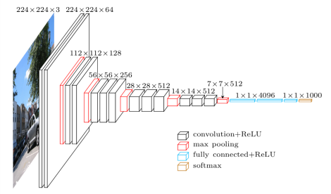
2. 定义一个卷积神经网络 下图是 VGG 的参考结构。但是我们这里随便定义一个 CNN 试试。
1
2
3
4
5
6
7
8
9
10
11
12
13
14
15
16
17
18
19
20
21
22
23
24
25
26
27
28
29
30
31
32
33
34
35
36
37
import torch.nn as nnimport torch.nn.functional as Fclass myNet (nn.Module ): def __init__ (self,in_size = 224 , in_channels = 3 , num_classes=2 ): super (myNet,self).__init__() self.conv1 = nn.Conv2d( in_channels, 15 ,3 ) self.conv2 = nn.Conv2d(15 , 75 ,4 ) self.conv3 = nn.Conv2d(75 ,150 ,3 ) self.conv4 = nn.Conv2d(150 ,300 ,3 ) self.conv5 = nn.Conv2d(300 ,300 ,3 ) self.fc1 = nn.Linear(7500 ,400 ) self.fc2 = nn.Linear(400 ,120 ) self.fc3 = nn.Linear(120 , num_classes) def forward (self,x ): x = F.max_pool2d(F.relu(self.conv1(x)), 2 ) x = F.max_pool2d(F.relu(self.conv2(x)), 2 ) x = F.max_pool2d(F.relu(self.conv3(x)), 2 ) x = F.max_pool2d(F.relu(self.conv4(x)), 2 ) x = F.max_pool2d(F.relu(self.conv5(x)), 2 ) x = x.view(x.size()[0 ],-1 ) x = F.relu(self.fc1(x)) x = F.relu(self.fc2(x)) x = self.fc3(x) return x use_cuda = True print ("CUDA Available: " ,torch.cuda.is_available())device = torch.device("cuda" if (use_cuda and torch.cuda.is_available()) else "cpu" ) net = VGG11(3 ,num_classes=2 ).to(device) net = myNet().to(device)
CUDA Available: True
3. 定义损失函数和优化器 让我们使用分类交叉熵损失(Classification Cross-Entropy)和带动量的 SGD(SGD with momentum)。
1
2
3
4
import torch.optim as optimcriterion = nn.CrossEntropyLoss() optimizer = optim.SGD(net.parameters(), lr=0.001 , momentum=0.9 )
4. 训练网络 我们只需在数据迭代器上循环,并将输入提供给网络和优化,就可以开始训练神经网络了
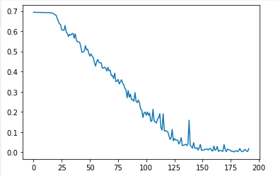
1
2
3
4
5
6
7
8
9
10
11
12
13
14
15
16
17
18
19
20
21
22
23
24
25
26
27
28
29
30
31
32
33
from tqdm import tqdmloss_plot = [] net.train() l = tqdm(range (192 )) for epoch in l: running_loss = 0.0 for i, data in enumerate (trainloader, 0 ): inputs, labels = data[0 ].to(device), data[1 ].to(device) optimizer.zero_grad() outputs = net(inputs) loss = criterion(outputs, labels) loss.backward() optimizer.step() running_loss += loss.item() if i % 100 ==99 : loss_plot.append(running_loss / 100 ) running_loss = 0.0 l.set_description(f'current loss: {loss_plot[-1 ]} ' ) print ('Finished Training' )plt.plot(loss_plot)
current loss: 0.017697893029380792: 100%|██████████| 192/192 [1:07:41<00:00, 21.15s/it]
Finished Training
[<matplotlib.lines.Line2D at 0x7fdadd729820>]
在实验中,我最开始发现 loss 曲线不下降,模型 train 不起来,如上图曲线的最开始的平坦的地方所示。我一度怀疑是什么地方错了,后来发现是 epoch 总数设置太少了。
这里可以保存一下训好的模型:
1
2
PATH = './fakeFace_{}.pth' .format (net.__class__.__name__) torch.save(net.state_dict(), PATH)
保存模型参考说明
5. 在测试数据上测试网络 我们已经通过训练数据集对网络进行了训练。但我们需要检查网络是否学到了任何东西。
第一步。让我们显示一个来自测试集的样本:
1
2
3
dataiter = iter (testloader) images, labels = dataiter.next () my_imgs_plot(images, labels)
使用训练好的神经网络判断是真脸还是假脸:
1 2 3 4 net.to('cpu' ) outputs = net(images)
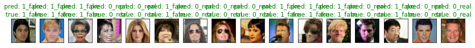
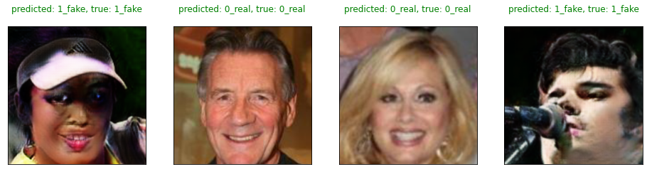
1 2 3 4 5 _, predicted = torch.max (outputs, 1 ) my_imgs_plot(images, labels,predicted)
发现都预测正确了(不正确的会标红),结果似乎相当不错。
让我们看看网络在整个测试集上的表现:
1
2
3
4
5
6
7
8
9
10
11
12
13
14
15
correct = 0 total = 0 net.eval () with torch.no_grad(): for data in tqdm(testloader): images, labels = data outputs = net(images) _, predicted = torch.max (outputs.data, 1 ) total += labels.size(0 ) correct += (predicted == labels).sum ().item() print (f'Accuracy of the network on the 10000 test images: {100 * correct // total} %' )
100%|██████████| 63/63 [00:15<00:00,  4.20it/s]

Accuracy of the network on the 10000 test images: 99.7 %
这看起来比随机选择要好得多,随机选择的准确率为 50%,而我们的模型达到了 99.7 %。
接着看看哪类表现良好,哪类表现不佳:
1 2 3 4 5 6 7 8 9 10 11 12 13 14 15 16 17 18 19 20 21 correct_pred = {classname: 0 for classname in class_names} total_pred = {classname: 0 for classname in class_names} with torch.no_grad(): for data in tqdm(testloader): images, labels = data outputs = net(images) _, predictions = torch.max (outputs, 1 ) for label, prediction in zip (labels, predictions): if label == prediction: correct_pred[class_names[label]] += 1 total_pred[class_names[label]] += 1 for classname, correct_count in correct_pred.items(): accuracy = 100 * float (correct_count) / total_pred[classname] print (f'Accuracy for class: {classname:5s} is {accuracy:.1 f} %' )
1
2
3
100%|██████████| 63/63 [00:15<00:00, 3.97it/s] Accuracy for class: 0_real is 100.0 % Accuracy for class: 1_fake is 99.4 %
但是通过 GPU 加速下仍一个小时的训练时间也太久了,99.7 %的准确率也不够满意,有没有更好的方法呢?
虚假人脸分类的迁移学习
本节参考:Transfer Learning for Computer Vision Tutorial — PyTorch Tutorials 1.11.0+cu102 documentation
实际上,很少有人训练整个卷积网络从头开始(随机初始化),因为很少有足够大的数据集。相反,这是很常见的在非常大的数据集上预训练 ConvNet(例如,ImageNet 包含 120 万张图像(包含 1000 个类别),然后使用 ConvNet 可以作为一个初始化或固定的功能提取器。
这两个主要的迁移学习场景如下所示:
ConvNet 作为固定特征提取器 :在这里,我们将冻结权重对于所有网络,除了最终完全连接的网络层最后一个完全连接的层将替换为新层使用随机权重,只对该层进行训练。微调 ConvNet :我们不是随机初始化,而是用预先训练好的网络初始化网络,比如在 imagenet 1000 数据集上接受培训。剩下的训练看起来也一样通常的
1
2
3
4
5
6
7
8
9
10
11
12
13
14
15
16
17
from __future__ import print_function, divisionimport torchimport torch.nn as nnimport torch.optim as optimfrom torch.optim import lr_schedulerimport torch.backends.cudnn as cudnnimport numpy as npimport torchvisionfrom torchvision import datasets, models, transformsimport matplotlib.pyplot as pltimport timeimport osimport copycudnn.benchmark = True plt.ion()
<matplotlib.pyplot._IonContext at 0x7fd0cccd90a0>
1. 读取数据 这里与上一节 基本相同。
通常,这是一个非常复杂的问题如果从零开始训练,就可以对小数据集进行概括。自从我们如果使用迁移学习,我们应该能够合理地概括好
1 2 3 4 5 6 7 8 9 10 11 12 13 14 15 16 17 18 19 20 21 22 23 24 25 26 27 28 29 data_transforms = { 'train' : transforms.Compose([ transforms.RandomResizedCrop(224 ), transforms.RandomHorizontalFlip(), transforms.ToTensor(), transforms.Normalize([0.485 , 0.456 , 0.406 ], [0.229 , 0.224 , 0.225 ]) ]), 'validation' : transforms.Compose([ transforms.Resize(256 ), transforms.CenterCrop(224 ), transforms.ToTensor(), transforms.Normalize([0.485 , 0.456 , 0.406 ], [0.229 , 0.224 , 0.225 ]) ]), } batch_size = 4 data_dir = './CNN_synth_testset_divided/' image_datasets = {x: datasets.ImageFolder(os.path.join(data_dir, x), data_transforms[x]) for x in ['train' , 'validation' ]} dataloaders = {x: torch.utils.data.DataLoader(image_datasets[x], batch_size=batch_size, shuffle=True , num_workers=4 ) for x in ['train' , 'validation' ]} dataset_sizes = {x: len (image_datasets[x]) for x in ['train' , 'validation' ]} class_names = image_datasets['train' ].classes device = torch.device("cuda:0" if torch.cuda.is_available() else "cpu" )
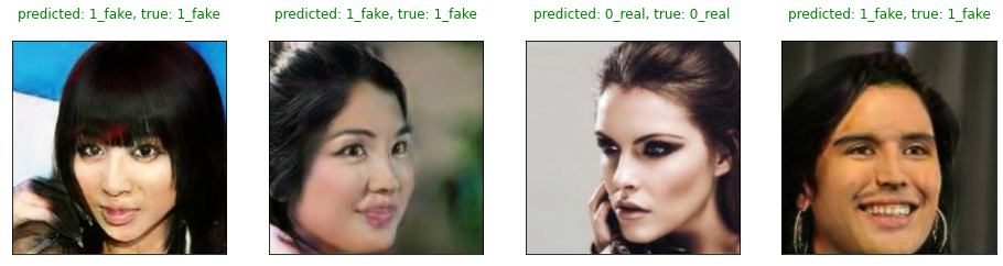
可视化一些图像 1 2 3 4 5 6 7 8 9 10 11 12 13 14 15 16 17 18 19 20 21 22 23 24 25 26 27 28 29 30 31 32 33 34 35 36 37 def imshow (inp, title=None ): """Imshow for Tensor.""" inp = inp.numpy().transpose((1 , 2 , 0 )) mean = np.array([0.485 , 0.456 , 0.406 ]) std = np.array([0.229 , 0.224 , 0.225 ]) inp = std * inp + mean inp = np.clip(inp, 0 , 1 ) plt.imshow(inp) if title is not None : plt.title(title) plt.pause(0.001 ) def my_imgs_plot (image, labels, preds=None ): cnt = 0 plt.figure(figsize=(16 ,16 )) for j in range (len (image)): cnt += 1 plt.subplot(1 ,len (image),cnt) plt.xticks([], []) plt.yticks([], []) if preds is not None : plt.title(f"predicted: {class_names[preds[j]]} , true: {class_names[labels[j]]} \n" ,color='green' if preds[j] == labels[j] else 'red' ) else : plt.title("{}" .format (class_names[labels[j]]), fontsize=15 , color='green' ) inp = image[j].numpy().transpose((1 , 2 , 0 )) mean = np.array([0.485 , 0.456 , 0.406 ]) std = np.array([0.229 , 0.224 , 0.225 ]) inp = std * inp + mean inp = np.clip(inp, 0 , 1 ) plt.imshow(inp) plt.show() inputs, classes = next (iter (dataloaders['train' ])) my_imgs_plot(inputs, classes)
2. 训练模型 现在,让我们编写一个通用函数来训练一个模型。
在下面的示例中,参数scheduler是来自的 LR scheduler 对象torch.optim.lr_scheduler。
1 2 3 4 5 6 7 8 9 10 11 12 13 14 15 16 17 18 19 20 21 22 23 24 25 26 27 28 29 30 31 32 33 34 35 36 37 38 39 40 41 42 43 44 45 46 47 48 49 50 51 52 53 54 55 56 57 58 59 60 61 62 63 64 65 66 67 from tqdm import tqdmdef train_model (model, criterion, optimizer, scheduler, num_epochs=25 ): loss_plot = [] since = time.time() best_model_wts = copy.deepcopy(model.state_dict()) best_acc = 0.0 for epoch in tqdm(range (num_epochs)): print (f'Epoch {epoch} /{num_epochs - 1 } :' ,end=' ' ) for phase in ['train' , 'validation' ]: if phase == 'train' : model.train() else : model.eval () running_loss = 0.0 running_corrects = 0 for inputs, labels in dataloaders[phase]: inputs = inputs.to(device) labels = labels.to(device) optimizer.zero_grad() with torch.set_grad_enabled(phase == 'train' ): outputs = model(inputs) _, preds = torch.max (outputs, 1 ) loss = criterion(outputs, labels) if phase == 'train' : loss.backward() optimizer.step() running_loss += loss.item() * inputs.size(0 ) running_corrects += torch.sum (preds == labels.data) if phase == 'train' : scheduler.step() epoch_loss = running_loss / dataset_sizes[phase] epoch_acc = running_corrects.double() / dataset_sizes[phase] loss_plot.append(epoch_loss) if phase == 'validation' and epoch_acc > best_acc: best_acc = epoch_acc best_model_wts = copy.deepcopy(model.state_dict()) time_elapsed = time.time() - since print (f'Training complete in {time_elapsed // 60 :.0 f} m {time_elapsed % 60 :.0 f} s' ) print (f'Best val Acc: {best_acc:4f} ' ) plt.plot(loss_plot) model.load_state_dict(best_model_wts) return model
可视化模型的预测 这是显示一些图像预测的函数
1
2
3
4
5
6
7
8
9
10
11
12
13
14
15
16
17
18
19
20
21
22
23
24
25
26
27
def visualize_model (model, num_images=8 ): was_training = model.training model.eval () images_so_far = 0 with torch.no_grad(): for i, (inputs, labels) in enumerate (dataloaders['validation' ]): inputs = inputs.to(device) labels = labels.to(device) outputs = model(inputs) _, preds = torch.max (outputs, 1 ) my_imgs_plot(inputs.cpu(),labels, preds) images_so_far += batch_size if images_so_far == num_images: model.train(mode=was_training) return model.train(mode=was_training)
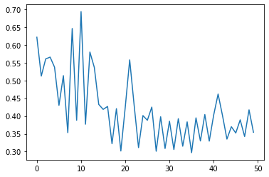
3. ConvNet 作为固定特征提取器 在这里,我们需要冻结除最后一层以外的所有网络。我们需要要设置requires_grad = False冻结参数,以便在backward()中不计算梯度。
1
2
3
4
5
6
7
8
9
10
11
12
13
14
15
16
17
model_conv = torchvision.models.resnet18(pretrained=True ) for param in model_conv.parameters(): param.requires_grad = False num_ftrs = model_conv.fc.in_features model_conv.fc = nn.Linear(num_ftrs, 2 ) model_conv = model_conv.to(device) criterion = nn.CrossEntropyLoss() optimizer_conv = optim.SGD(model_conv.fc.parameters(), lr=0.001 , momentum=0.9 ) exp_lr_scheduler = lr_scheduler.StepLR(optimizer_conv, step_size=7 , gamma=0.1 )
训练和评估 在 CPU 上,与之前的场景相比,这将花费大约一半的时间。这是预期的,因为大多数情况下不需要计算梯度,然而,forward 确实需要计算。
1
2
3
4
model_conv = train_model(model_conv, criterion, optimizer_conv, exp_lr_scheduler, num_epochs=25 ) PATH = './fakeFace_tf_{}.pth' .format (model_conv.__class__.__name__) torch.save(model_conv.state_dict(), PATH)
100%|██████████| 25/25 [07:15<00:00, 17.42s/it]

validation Loss: 0.3544 Acc: 0.8430
Training complete in 7m 15s
Best val Acc: 0.880000
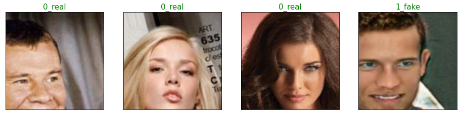
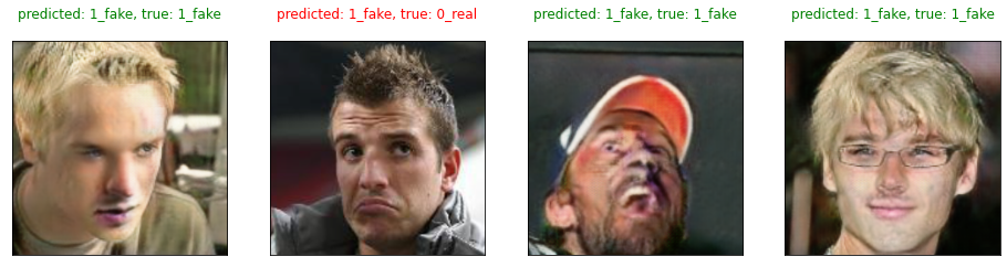
1
2
3
4
visualize_model(model_conv) plt.ioff() plt.show()
发现仅训练全连接层的话效果不太好,我们再试试对所有产生 Fine-tuning 的方法。
4. Fine-tuning - 微调网络 加载预训练模型并重置最终完全连接的层。
1
2
3
4
5
6
7
8
9
10
11
12
13
14
15
model_ft = models.resnet18(pretrained=True ) num_ftrs = model_ft.fc.in_features model_ft.fc = nn.Linear(num_ftrs, 2 ) model_ft = model_ft.to(device) criterion = nn.CrossEntropyLoss() optimizer_ft = optim.SGD(model_ft.parameters(), lr=0.001 , momentum=0.9 ) exp_lr_scheduler = lr_scheduler.StepLR(optimizer_ft, step_size=7 , gamma=0.1 )
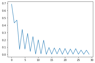
训练和评估 在 GPU 上,只需不到 10 分钟
1
2
model_ft = train_model(model_ft, criterion, optimizer_ft, exp_lr_scheduler, num_epochs=15 )
100%|██████████| 15/15 [10:20<00:00, 41.38s/it]

validation Loss: 0.0028 Acc: 1.0000
Training complete in 10m 21s
Best val Acc: 1.000000
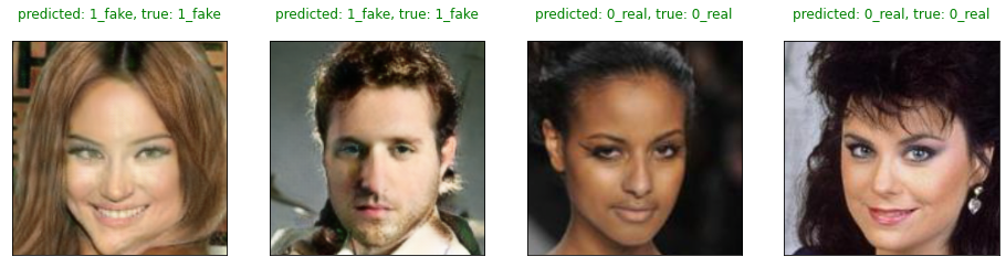
可以发现正确率达到了 100%。
1 visualize_model(model_ft)
参考 【学习笔记】如何理解 transforms.Normalize((0.5, 0.5, 0.5), (0.5, 0.5, 0.5))])_GRIT_Kael 的博客-CSDN 博客_transforms.normalize 参数
Autograd mechanics — PyTorch master documentation
(beta) Quantized Transfer Learning for Computer Vision Tutorial — PyTorch Tutorials 1.11.0+cu102 documentation
Transfer Learning for Computer Vision Tutorial — PyTorch Tutorials 1.11.0+cu102 documentation